How Classical and Quantum Computers Search a Maze
/ 10 min read
Table of Contents
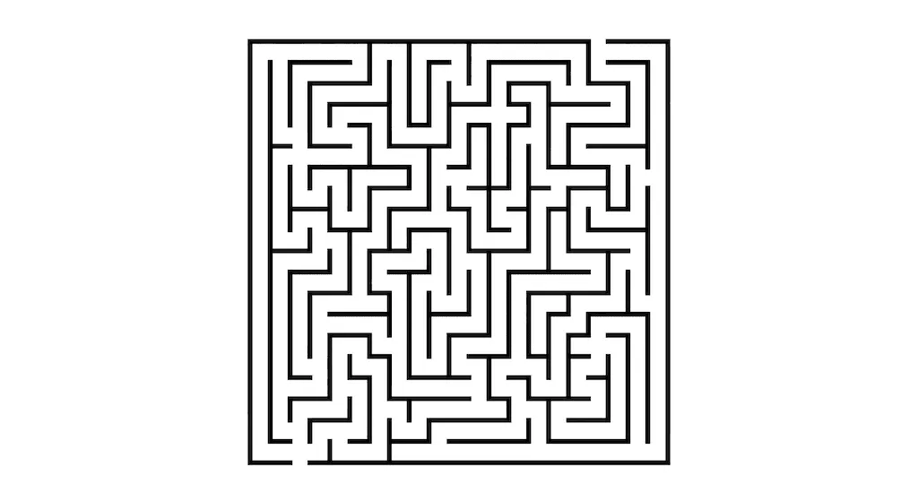
Imagine a maze. There’s a start, an exit, and a tangle of corridors and dead ends in between. Finding the way through is one of the oldest problems in computer science, and it turns out to be a surprisingly clean way to see what actually separates a quantum computer from the laptop on your desk.
The short version: a classical computer walks the maze, and a quantum computer makes the wrong paths cancel each other out. Let’s unpack what that really means — and where the popular “tries all paths at once” story is misleading.
How a classical computer searches
A classical computer explores a maze by trying candidate paths. The standard algorithms — depth-first search, breadth-first search, A* — all share the same basic character: they walk down a branch, and if it dead-ends, they back up and try the next one.
- Depth-first search plunges as far down one corridor as it can, backtracking only when it hits a wall.
- Breadth-first search explores all paths of length 1, then all of length 2, and so on, guaranteeing the shortest route.
- A* adds a heuristic — a guess about which direction points toward the exit — to explore promising branches first.
These get smarter about which paths to check and in what order, and some — breadth-first search, for one — fan out across a whole frontier of paths at once rather than truly one at a time. But none of them has a way to make wrong answers cancel. They can prune, reorder, and even parallelize the checking, yet every wrong candidate still has to be ruled out on its own; there is no global mechanism that lets the dead ends suppress each other. That absence — not sequential-versus-parallel — is the real line between classical and quantum search. When a maze has many branching points the number of possible paths grows exponentially, and in the worst case there’s no escaping that the work scales with the number of candidates you have to eliminate.
How a quantum computer searches
A quantum computer does not literally try every path simultaneously, even though that’s the line you’ll read everywhere. The reality is more subtle and more interesting.
A quantum computer puts the system into a superposition over many possible paths at once, then uses interference to make the wrong paths cancel out while the right path’s contribution builds up. Quantum states are described by amplitudes — numbers that can be positive or negative — and the probability of measuring any given state is its amplitude squared. Because amplitudes carry a sign, they can add together or cancel, exactly like waves.
The catch is that you only ever get one measurement. You can’t peek at the superposition and read off all the paths. So the entire game is arranging the interference so that, when you finally measure, you’re overwhelmingly likely to read out the correct answer. The parallelism is real, but it’s fragile — it has to be carefully engineered to survive collapse into a single result.
Recast as unstructured search — find the one valid path among many candidates, with no clue which is which beyond what a checker tells you — the relevant tool is Grover’s algorithm. (A real maze has structure that classical graph search exploits; deliberately throwing that structure away is what turns it into a clean illustration of Grover, not how you’d actually solve a small maze.)
Encoding a maze as a search problem
Before Grover can help, the maze has to be expressed as a search problem.
Think of the maze as a graph: each cell or junction is a node, and each open passage between two cells is an edge. A path is a sequence of moves from the start to the exit.
To make this something a quantum algorithm can chew on, you encode a candidate path as a bit string. Suppose at every junction you can move in one of four directions, and a complete path is at most moves long. Each move needs 2 bits (4 directions = 2 bits), so a full candidate path is a string of bits. The total space of candidate paths is:
Most of these strings are nonsense — they walk into walls, wander off the grid, loop forever, or never reach the exit.
Now you need an oracle: a function that takes a candidate path and returns 1 if it’s a valid solution and 0 otherwise. The key insight is that checking a given path is easy — you just trace it and see whether it goes start-to-exit without crossing a wall. The hard part is that there are candidates and you have no idea in advance which one the oracle will accept.
One practical caveat the tidy picture hides: on real hardware this oracle has to be built as a reversible circuit — every step undoable, no information discarded along the way — which adds engineering overhead, though it doesn’t change the asymptotic speedup.
That structure — “find the one needle the oracle marks, among haystack items” — is precisely what Grover’s algorithm is built to solve.
- Classically: you feed candidates to the oracle one by one, expecting to test about before you stumble on the answer.
- With Grover: you find it in roughly steps.
Two things that “roughly steps” quietly hides. Each step is one oracle call plus one diffusion operator, and an oracle call isn’t free — tracing a length- path costs about — so the honest runtime is . Grover cuts the number of oracle calls from about to about ; it doesn’t make each call cheaper. And this assumes a single valid path. If there are of them, Grover finds one in about steps — more needles, fewer iterations.
How Grover’s interference builds up the answer
Here’s the mechanism, step by step.
Step 1 — Equal superposition
Start with all candidate paths in equal superposition. Every path has the same amplitude:
If you measured now, you’d get a random path. Useless — the right answer is just one in .
Step 2 — The oracle flips the sign
The oracle doesn’t boost the winning path’s probability directly. Instead it flips the sign of the winner’s amplitude, leaving every other amplitude untouched. The winner now sits at while everyone else stays at .
Its probability (amplitude squared) hasn’t changed at all — you’ve marked it invisibly, purely by sign.
Step 3 — Inversion about the mean
This is the clever move, often called the diffusion operator. You compute the average of all the amplitudes, then reflect every amplitude across that average. Each value becomes:
Watch what happens. Because the winner is negative and everyone else is positive, the average sits slightly below the positive cluster. Reflecting the positive paths across that average nudges them down a little. But reflecting the negative winner across the average flings it way up to a large positive value. In a single step, the winner’s amplitude has grown while everyone else’s has shrunk.
Step 4 — Repeat (but not too much)
Each oracle-plus-diffusion cycle rotates probability toward the winner. Geometrically, it’s literally a rotation: the state vector turns by a fixed small angle toward the answer on each iteration. After about
iterations, the winner’s amplitude is close to 1, and a measurement returns the correct path with high probability.
The subtlety people get wrong: you have to stop at the right time. Because it’s a rotation, running past the optimal point rotates you past the answer, and the success probability starts falling again. More iterations is not better — Grover overshoots. That’s a genuine departure from classical search, where extra effort never hurts.
Watching it happen: a worked example with N = 16
Let’s make this concrete with a small maze of candidate paths, where path #0 is the correct one. The optimal number of iterations is .
These aren’t hand-waved figures — each row is the exact Grover rotation. With one correct path out of , define . After iterations the winner’s amplitude is , each of the wrong paths sits at , and the success probability is . For , , and the rotation lands on clean values — and — which is where the table comes from.
| Iteration | Winner amplitude | Each wrong amplitude | P(winner) | P(each wrong) |
|---|---|---|---|---|
| 0 | 0.2500 | 0.2500 | 6.25% | 6.25% |
| 1 | 0.6875 | 0.1875 | 47.3% | 3.52% |
| 2 | 0.9531 | 0.0781 | 90.8% | 0.61% |
| 3 | 0.9805 | −0.0508 | 96.1% | 0.26% |
| 4 | 0.7627 | −0.1670 | 58.2% | 2.79% |
| 5 | 0.3542 | −0.2415 | 12.6% | 5.83% |
| 6 | −0.1428 | −0.2556 | 2.04% | 6.53% |
Reading the table:
- Iteration 0 — everything is flat. All 16 paths sit at amplitude 0.25, each with a 6.25% chance (). Measuring now is a coin-toss across all paths.
- Iteration 1 — after one cycle, the winner jumps to 0.6875 and each wrong path drops to 0.1875. The winner alone is already at 47%, nearly even odds against all 15 competitors combined.
- Iteration 2 — winner at 0.95; the 15 wrong paths barely register. Already 90.8%.
- Iteration 3 — the peak. The winner hits 96.1%, exactly where the formula predicted. This is where you measure.
- Iterations 4–6 — the overshoot. Past the peak, the rotation keeps turning past the answer. The winner’s amplitude falls, goes negative by iteration 6, and its probability collapses to 2% — worse than where you started.
You can see the rotation directly in the signs: the winner climbs to its maximum, then the amplitudes start flipping negative as the state vector swings past the target. That’s why “just run it longer” actively hurts. A quantum search has a correct stopping time; a classical search never does.
So how much faster is it, really?
The honest answer is quadratically faster — not exponentially.
If a classical search through possibilities takes roughly steps, Grover finds the marked item in about steps. A maze that takes a million classical checks might take around a thousand Grover iterations.
A quick way to feel the speedup: each Grover iteration rotates the state by , which for large is close to . You start near angle and need to turn the state to about radians, so it takes about iterations rather than checks.
| Search space | Classical (≈ ) | Grover (≈ ) |
|---|---|---|
| 16 | 8 | 3 |
| 1,000,000 | 500,000 | ~785 |
The gap at looks modest. At a million, it’s the difference between half a million checks and a few hundred iterations. But notice it’s versus , not exponential-versus-polynomial. For this kind of unstructured search, quantum computing helps a great deal — but it doesn’t make genuinely hard problems trivially easy.
Two honest caveats
It’s worth being clear-eyed about what this does and doesn’t deliver.
First, most real mazes have structure. Good classical algorithms — A* with a sensible heuristic, for instance — exploit that structure aggressively. Grover’s quadratic speedup assumes unstructured search, where you have no clue which candidate is the answer beyond what the oracle tells you. A quantum computer is not automatically better than a smart classical algorithm on a structured maze.
Second, today’s hardware can’t do this for real. Current quantum machines are too noisy to beat a laptop on a problem like this. The advantage here is theoretical and asymptotic — a statement about how the work scales as the problem grows, not something you’d observe on present-day devices.
The takeaway
A classical computer searches a maze by trying paths, one after another, backtracking from dead ends. A quantum computer never “tries” paths in that sense at all. It places every candidate into superposition and then, using nothing more than the oracle’s sign-flip and a reflection about the mean, sloshes probability amplitude around until it concentrates on the correct path — in about steps instead of .
It never knows the answer along the way. The geometry of those two reflections simply happens to funnel near-certainty onto the marked state. And if you let it run too long, that same geometry funnels the certainty right back out again.